TL;DR: Does the next-token logit track the conditional or the joint probability of the whole sequence?

I had an invisible gorilla moment while reading a paper. Even though the paper interprets the gorilla in a way I’m not in agreement with, in helping me notice something so basic that was staring at me all along, the paper led me closer to clarity.

The paper is called “Spilled Energy in Large Language Models” by Robert et al., 2026¹ which proposes a way to predict whether or not a generated token is hallucinated. The proposal is simple and cute: when you generate a token, if you’re suspicious of it, take the corresponding logit of that token as $\tt{Term} 1$; feed the suspicious token in and proceed to the next step, where you take the denominator of the softmax probability as $\tt{Term 2}$. If $\tt{Term 2}$ is much smaller than $\tt{Term 1}$, your model has likely hallucinated. This difference quantity is what they call as “Spilled Energy”.

Specifically, if $f( \tt{token} ; \tt{context} )$ is my language model’s logit on a token given a context as input, if $x$ is my suspicious token, and $y’$ some next token candidate (I’ll save the symbol $y$ for later!), then:

\[\begin{equation} \textrm{Spilled Energy} = \underbrace{f(x ; \tt{context})}_{\tt{Term1}} - \underbrace{\log \sum_{y'} \exp(f( y' ; {\tt context}, x))}_{\tt{Term2}} \end{equation}\]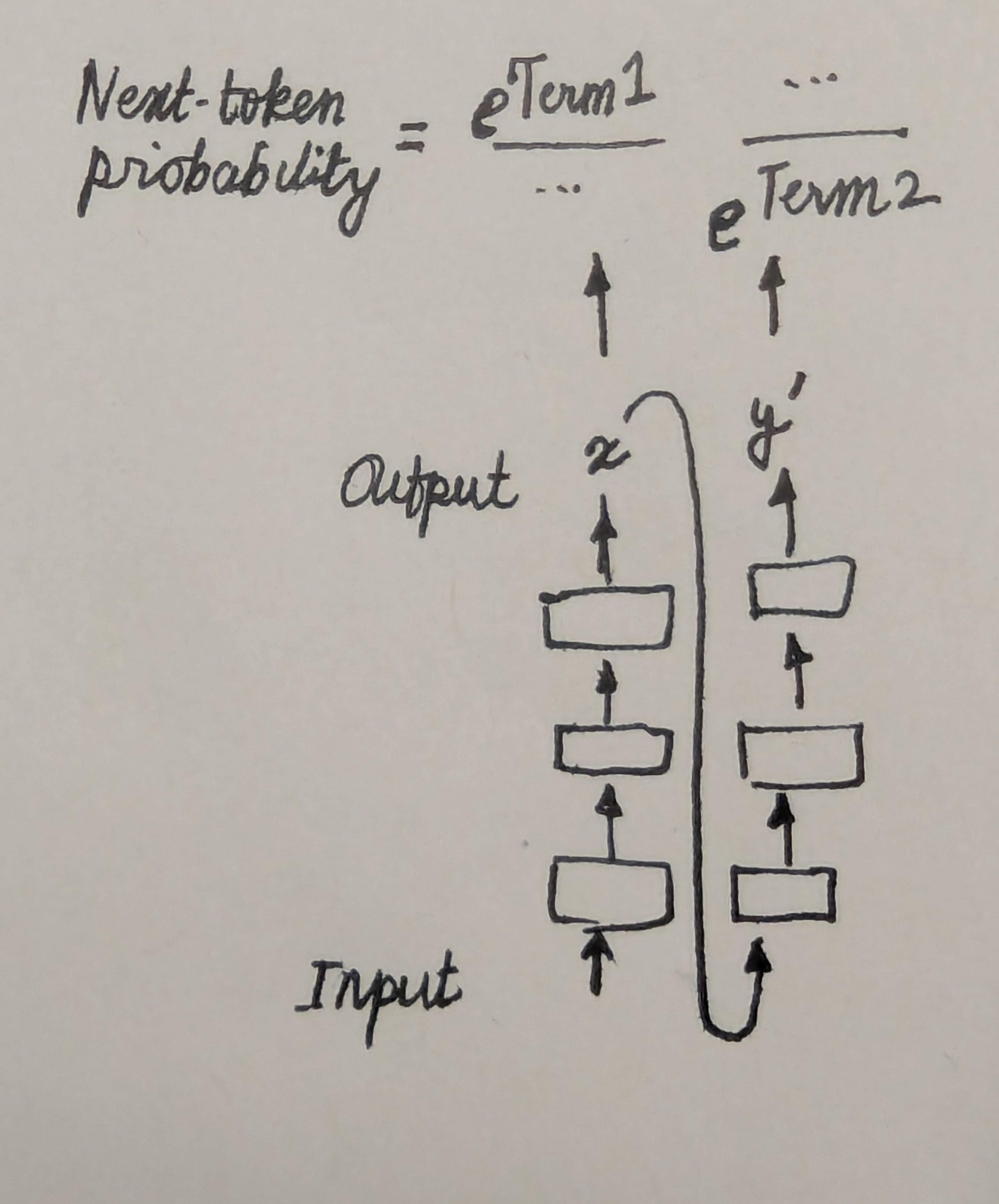

First things first, I made sure this smelled good: ${\tt Term 1}$ reflects the enthusiasm² of the model in predicting the suspicious token, ${\tt Term 2}$ the enthusiasm of the model in continuing that train of thought for one more step, summed over all possible continuations. If the model abruptly turns unenthusiastic, it means that the model has found itself in a grave it enthusiastically dug one step ago. Makes sense. But is this handwavy justification all there is to it?

The paper’s interpretation

The paper offers a tighter justification. The joint probability that the model assigns to a sequence must be decomposable into next-token probabilities, a fact the reader should be able to blurt out in sleep:

\[\require{color} \begin{align} p({\tt context}, x, y) & = p({\tt context}) \cdot p(x | {\tt context}) \cdot p(y| {\tt context}, x) \\ & = p({\tt context}) \cdot \frac{\colorbox{silver}{$\color{black} p({\tt context}, x )$}}{p({\tt context})} \cdot \frac{p({\tt context}, x, y)}{\colorbox{silver}{$\color{black} p({\tt context}, x )$}} \label{eq:dec1} \end{align}\]

Then comes the main claim: the next-token-predicting language model has been designed to capture these very next-token quantities; which means ideally every numerator and its subsequent denominator, as estimated by the model, should cancel out (${\tt Term1}$ and ${\tt Term 2}$). Yet, the claim goes, nothing in a language model imposes this constraint on its estimates!

Specifically if we let $\hat{p}$ be the model’s assigned probability to a sequence, we can write it in a way that resembles Eq \eqref{eq:dec1}:

\[\begin{align} \hat{p}({\tt context}, x, y) & = p({\tt context}) \cdot \frac{ \overbrace{ \colorbox{silver}{$\color{black}\exp{f(x; \tt{context})}$ }}^{\propto \exp({\tt Term1})}}{\sum_{x'} \exp{f(x'; {\tt context})}} \cdot \frac{ \exp{f(x; \tt{context})}}{\underbrace{ \colorbox{silver}{$\color{black}\sum_{y'} \exp{f(y'; {\tt context}, x)}$} }_{\propto \exp(\tt Term2)}} \label{eq:energy} \\ \end{align}\]

Now, the claim goes on to “superimpose” \eqref{eq:energy} over \eqref{eq:dec1}, implying that every term in the former corresponds to the latter. If this was true, then ${\tt Term1}$ must match ${\tt Term2}$ for their corresponding terms match in Eq \eqref{eq:dec1}. When these Terms do not match in practice, we are to conclude that there is profoundly erratic behavior within the model, manifesting as hallucinations.

My interpretation

This disturbed me: how had I missed a gorilla hiding in an object I had stared at for weeks at one point?³ A further staring contest resolved this confusion—only somewhat though, as you’ll find at the end of this post. (But, before you proceed any further, I recommend stepping away from this to think for yourself.)

(Welcome back!) Here’s the resolution: I had just never done the superimposition this way (and it seems, I wouldn’t do it this way). I had always, with certainty, superimposed Eq $\eqref{eq:energy}$ over a decomposition different from Eq $\ref{eq:dec1}$:

\[\begin{align} p({\tt context}, x, y) & = p({\tt context}) \cdot \frac{ \colorbox{silver}{$\color{black}p(x | {\tt context} )$} }{\sum_{x'} p({x' | \tt context})} \cdot \frac{p(y | {\tt context}, x)}{ \colorbox{silver}{$\color{black}\sum_{y'} p(y' | {\tt context}, x)$} } \label{eq:dec2} \end{align}\]

In other words, I had always viewed the logits as representing how likely the next-token was, rather than how likely the whole sequence was! In this expression, the numerator and the denominator do not match (the denominator is always $1$ but the numerator isn’t!). We can also think in terms of the proportionality constants. In the paper’s, there is some global constant $Z$ such that if you divide each energy/logit term in every numerator and denominator of \eqref{eq:energy} by $Z$, you get back the terms in \eqref{eq:dec1}. In my interpretation, although $\tt{Term1}$ is proportional to the numerator of \eqref{eq:dec2}, the proportionality constant is only local to token $x$’s probability; likewise $\tt{Term2}$ is proportional to its denominator, with a constant local to $y$’s probability. (These constants are the respective denominators themselves.)

To me this was the obvious interpretation: we train a model on the next-token loss with the hope that it learns how good/bad that token is, with no care for how likely the input sequence itself is, and this is what the logits capture.

It’s actually not that clear which interpretation is correct.

Continuing the staring contest bit more had me questioning this all over again. If indeed the logits are not to be interpreted as representing the joint probability, and so, ${\tt Term2}$ is indeed unconcerned about what preceded the $y$ token, why does the spilled-energy metric even work?

My explanation is this. While the next-token loss does stipulate what the probabilities must be—the next-token conditionals—the logit magnitudes themselves are underdetermined. Usually, in gradient-descent-trained models, if something is free to move as it pleases, it moves gracefully, and I suspect we find this grace in the logits too. Consider ${\tt Term2}$. On seen contexts, a well-trained generative model’s logits will be forced to spike up (to $\infty$) on the seen next-token and spike down (to $-\infty$) on all other next tokens, and so the “total energy” in ${\tt Term 2}$ would explode. On completely bizarre contexts (say, due to our suspicious $x$ token), the next-token logits are “free to be what they want” and so, we may expect them to largely remain unenthusiastic (blunting ${\tt Term 2}$). In between these extremes, as we get closer and closer to the training manifold, we can expect the logits to be more and more enthusiastic on some next-tokens. This way, it seems that the total energy term in ${\tt Term 2}$ is indeed indicative of the how likely the $({\tt context}, x, y)$ sequence is!

If you think about it, you’ll find that this argument can be applied to even make boring image classifiers appear as though they are models of the input distribution: when your input image is garbage, the logits are likely tiny in magnitude; when your input image is realistic, some of the logits are highly positive!

Thus, do the logits represent the joint probability after all? Now I do not mean to say that these logits are exactly representative of the joint probability: on some reasonable inputs, the next-token logits may be unenthusiastic purely due to poor learning, causing under-confidence on its next-token prediction. But what of a model that has perfectly learned the next-token conditionals? Is its logits nicely representative of the joint distribution?

The open question

Surely, next-token probabilities of a model indeed only model the conditionals; but due to the implicit bias of gradient descent, it’s possible that the next-token logits reflect, to some extent, the joint probability of $({\tt context}, x)$, with some additional factors corresponding to the next-token confidence itself. Is this just a feel-good empirical observation? Or is it possible to give this a mathematical form? Has someone already done this?

(Maybe this gorilla was always visible and many knew of it; or maybe this gorilla is just a figment of my imagination; but for the time being, I will enjoy the feeling of having noticed it.)

---

Footnotes